Tutorial: Ringer and Calmodulin
This tutorial covers using Ringer to identify unmodeled, alternate conformations in the calcium-signaling protein Calmodulin (CaM).
1) Preparing the Coordinate and Structure Factor Files
The structure for calcium-bound CaM has been solved previously (Wilson MA et al. J. Mol. Biol. 301 (2000): 1237-1256) at 1.0Å resolution with an R-value of 0.13. The coordinate file and structure factors can be downloaded from the Protein Data Bank (PDB Code 1EXR).
The structure factors must be converted into an electron density map. A typical procedure might be:
a) Add hydrogens to the model using phenix.ready_set
b) Convert the structure factor file to MTZ format using phenix.cif_as_mtz (distributed with Phenix)
c) Run refinement using phenix.refine
d) Convert the 2FOFCWT and PH2FOFCWT columns into a map in CCP4 format using fft, with these commands:echo labin F1=2FOFCWT PHI=PH2FOFCWT | fft hklin phenix_001.mtz mapout ffted.map
echo xyzlim cell | mapmask mapin ffted.map mapout cell.mapuse the file "cell.map" a full unit cell so that chimera doesn't get confused in space groups like R3 or H3.
After this procedure, the R-value for CaM was 0.14. Here is the coordinate file (1EXR.pdb) and map file (1EXR_2FoFc.map) that is used in the next step.
2. Running Ringer
We are now ready to run Ringer. Here is the input file (ringer.in). Ringer can then be run using the following command:
$RINGER/ringer/ringer -i ringer.in
ringer.in
pdb_name 1EXR.pdb
map_type sigma
skip_multi_conf on
atom_sample_type dynamic
chi_sample_degree 10
lower_sigma_cutoff 0.3
upper_sigma_cutoff off
write_plot on
write_chi2chi1 off
write_peak_list on
verbose_outfile_prefix ringer
We start by telling Ringer where to find the map and pdb file. We also set the map type, in this case a sigma map. If you have run the END/RAPID procedure and wish to use that map instead, you should set the map type to be 'volume'.
In this example, we are interested in finding the unmodeled, alternate conformations. Therefore, we skip over the residues that already have alternate conformations built in by turning on skip_multi_conf. We look below the standard 1.0 sigma cutoff to identify low population conformations by setting lower_sigma_cutoff to 0.3 sigma.
Finally, we have Ringer print out the raw data for the sigma vs. chi angle plots for serine and aspartic acid side chains. We also print out the list of peaks that Ringer identifies above the 0.3 sigma cutoff.
NOTE: For more information on Ringer options, please see User Parameters in the Ringer Manual
3. Looking at Ringer Output
Based on the parameters set above, Ringer produces a number of output files. The general output file, ringer.out, gives a description of the run. It starts by listing all of the parameters that were used in the run. If a parameter is not declared by the user in the input file (eg atom_sample_type), the default value that was used in the run is printed. Next, it lists the residues that are not analyzed by Ringer, in this case the calcium ions. The side chains that are skipped because they have alternate conformations are also listed. The file then lists any sampled atoms that are not centered in an electon density peak. Finally, the output file then lists some statistics about the run including the total number side chains in each category (eg 65 side chains unbrached at chi 1).
The raw data needed to plot the sigma vs chi angle plots is printed in ringer.signal_plot.txt. The first line lists the residue names and sampled chi angle. This particular residues of interest can be parsed from the file or plotted using the plotting accessory.
The lists of peaks identified above the 0.3 sigma cutoff is printed in ringer.ala_peaklist.txt (alanines), ringer.ubchi1_peaklist.txt (residues unbranched at chi1), ringer.ring_peaklist.txt (ring residues), ringer.ubchi2_peaklist.txt (residues unbranched at chi2), ringer.chi3_peaklist.txt (residues unbranched at chi3), and ringer.chi4_peaklist.txt (residues unbranched at chi4). All files list the residue name and corresponding peaks, listed in order of sigma density. Each peak is described by the sigma value and the chi angle location followed by a semi-colon.
4. Analyzing the Output
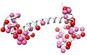
The peak lists can be mapped onto the model to indicate where the alternate conformations are located:
The peak lists can be used in combination with the sigma vs chi angle plots to identify and build alternate conformations into the map electron density.
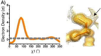
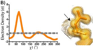
conformations are shown superimposed on the electron density at 1 sigma (solid) and 0.3 sigma (mesh). Arrows indicate areas of interest in electron density. Ringer plots of electron density (sigma) versus chi1 angle for two representative residues (A) Ser38 (B) Asp22. Gray dashed line indicates 0.3 sigma.